Like SVMs, Decision Trees are versatile Machine Learning algorithms that can perform both classification and regression tasks, and even multioutput tasks. In this blog, I will introduce Decision Trees with following point:
- Training and visualizing a Decision Tree
- The CART training algorithm
- Estimating class probabilities
- Regression
Training and visualizing a Decision Tree
To understand Decision Trees, let’s just build one and take a look at how it makes predictions.
>>> from sklearn.datasets import load_iris
>>> from sklearn.tree import DecisionTreeClassifier
>>>
>>> iris = load_iris()
>>> X = iris.data[:, 2:] # petal length, petal width
>>> y = iris.target
>>>
>>> tree_clf = DecisionTreeClassifier(max_depth=2)
>>> tree_clf.fit(X, y)

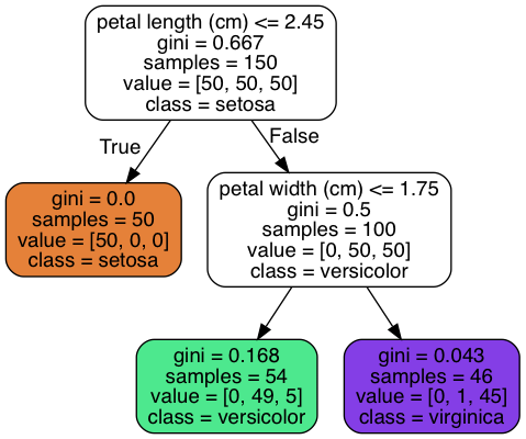
How to classify a flower with the classification decision tree above? Imagine that you find a flower whose petal length is 3 cm and petal width is 2 cm. Now we start at the root node (depth 0, at the top), this node asks whether the flower’s petal length is smaller than 2.45 cm. In our case, it is, so we move down to the root’s right child node (depth 1, right). Then we judge that the petal width is greater than 1.75 cm, so we continue to move down to the root’s right child node (depth 2, right). In this case, it is a leaf node, which means that it doesn’t have any children nodes, so it does not ask any questions. The decision tree predicts that your flower is Iris-Virginica.
A node’s gini attributes measures its impurity: a nodes is pure if all
training instances that it applies to belong to the same class (gini=0). A
node’s samples attributes counts how many training instances it applies to. A
node’s value attributes tells us how many training instances of each class
this node applies to.
The CART training algorithm
Scikit-Learn uses the Classification And Regression Tree (CART) algorithm to train decision trees. The algorithm first splits the training set into two subsets using a single feature k and a threshold t_k (e.g. “petal width <= 2.45 cm”). How does it choose k and t_k? It searches for the pair (k, t_k) that produces the purest subsets.
CART cost function for classification:

where G_left/right measures the impurity of the left/right subset, m_left/right is the number of instances in the left/right subset.
Once it successfully split the training set into two, it splits the subsets
using the same logic; it stops recursing once it reaches the maximum depth. We
can control hyperparameters for stopping conditions (min_* and max_*), we
can also regularize the model with them. Reducing max_depth will reduce the
risk of overfitting.
Estimating class probabilities
A decision tree can estimate the probability that an instance belongs to a particular class k.
>>> tree_clf.predict_proba([[5, 1.5]])
array([[0.        , 0.90740741, 0.09259259]])
>>> tree_clf.predict([[5, 1.5]])
array([1])
If a flower’s petal is 5 cm long and 1.5 cm wide, it is predicted as an Iris-Versicolor.
Regression
Decision Trees are also capable for performing regression tasks:
from sklearn.tree import DecisionTreeRegressor

tree_reg = DecisionTreeRegressor(max_depth=2, random_state=42)
tree_reg.fit(X, y)

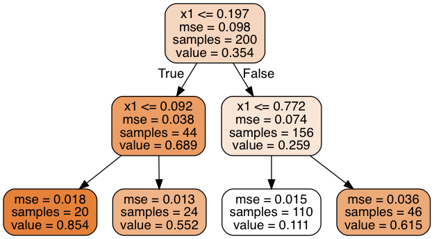
The main difference between the regression tree and classification tree is that instead of predicting a class in each node, it predicts a value. The algorithm splits each region in a way that makes most training instances as close as possible to that predicted value.
The CART algorithm works mostly the same way as classification task, instead of trying to split the training set in a way that minimizes impurity, it now tries to split the training set in a way that minimizes MSE.
CART cost function for regression:

Conclusion
In this blog, I introduced how CART algorithm works for classification and regression Decision Tree, how we understand and predict with the Decision Tree. Hope it’s useful for you.
Reference
- Aurélien Géron. 2017. “Chapter 6 Decision Trees” Hands-On Machine Learning with Scikit-Learn & TensorFlow p 169-180
- jplenio, “Tree nature wood sunset light”, pixabay.com. [Online]. Available: https://pixabay.com/photos/tree-nature-wood-sunset-light-3822149/