A Support Vector Machine (SVM) is a very powerful and versatile Machine Learning model, capable of performing linear or nonlinear classification and regression. It is one of the most popular models in Machine Learning. SVMs are suited for classification of complex but small- or medium-sized datasets. In this blog, I will talk about SVM with the following points:
- What is Support Vector Machine (SVM)?
- Linear SVM Classification
- Nonlinear SVM Classification
- SVM Regression
What is Support Vector Machine (SVM)?
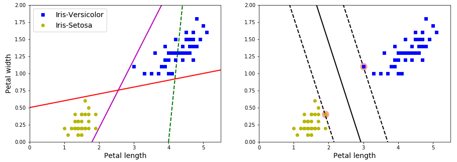
The fundamental idea behind SVMs is best explained with some figures. As showing above, the left plot presents the decision boundaries of three possible linear classifiers. The model whose decision boundary is shown by dashed line is bad that it cannot separate classes clearly. Other two models work perfectly on the training set, but since their boundaries are so close to the instances that risk not performing well on new instances. On the contrary, in the right plot, the solid line represents the decision boundary of an SVM classifier, this line not only separates the two classes but also stays far away from the training instances. You can think of an SVM classifier as fitting the widest possible street between the classes, the instances located on the edge of the street are support vectors.
Linear SVM Classification
The SVM classifier above presents a linear SVM classification. If we strictly impose that all instances be off the street, this makes it sensible to outliers and only works if the data is linearly separable. To avoid it, we need to find a good balance between keeping the street as large as possible and limiting the margin violations, which called soft margin classification.
In Scikit-Learn’s SVM classes, we can control the balance with hyperparameter
C: a smaller C value leads to a wider street but more margin violations. If
your SVM model is overfitting, you can try to regularize it by reducing C.
>>> import numpy as np
>>> from sklearn import datasets
>>> from sklearn.pipeline import Pipeline
>>> from sklearn.preprocessing import StandardScaler
>>> from sklearn.svm import LinearSVC
>>>
>>> iris = datasets.load_iris()
>>> X = iris['data'][:, (2, 3)]
>>> y = (iris['target'] == 2).astype(np.float64)
>>>
>>> svm_clf = Pipeline([
...         ('scaler', StandardScaler()),
...         ('linear_svc', LinearSVC(C=1, loss='hinge', random_state=42)),
...     ])
>>> svm_clf.fit(X, y)
>>> svm_clf.predict([[5.5, 1.7]])
array([1.])
The codes above loas the iris datasets, scales the features and trains a linear SVM model to detect Iris-Virginica flowers.
Nonlinear SVM Classification
Although linear SVM classifiers are efficient, many datasets are even close to being linearly separable.
In order to handle nonlinear datasets, we can add more features, such as polynomial features, like the codes below.
>>> from sklearn.datasets import make_moons
>>> from sklearn.pipeline import Pipeline
>>> from sklearn.preprocessing import PolynomialFeatures
>>>
>>> polynomial_svm_clf = Pipeline([
...         ('poly_features', PolynomialFeatures(degree=3)),
...         ('scaler', StandardScaler()),
...         ('svm_clf', LinearSVC(C=10, loss='hinge', random_state=42))
...     ])
>>>
>>> polynomial_svm_clf.fit(X, y)
Adding polynomial features is simple to implement and can work well with all sorts of Machine Learning algorithms. But at a low polynomial degree it cannot deal with very complex datasets, and with a high polynomial degree it creates a huge number of features, which makes the model too slow.
Luckily, we can apply kernel trick, which makes it possible to get the same result as if you added polynomial features, without actually having to add them.
>>> from sklearn.svm import SVC
>>>
>>> poly_kernel_svm_clf = Pipeline([
...         ("scaler", StandardScaler()),
...         ("svm_clf", SVC(kernel='poly', degree=3, coef0=1, C=5))
...     ])
>>> poly_kernel_svm_clf.fit(X, y)
If your model is overfitting, you might want to reduce the polynomial degree;
conversely, if it is underfitting, you can try to increase it. The
hyperparameter coef0 controls how much the model is influenced by high-degree
polynomial vs. low-degree polynomials.
SVM Regression
Instead of trying to fit the largest possible street between two classes, SVM
Regression tries to fit as many instances as possible on the street while
limiting margin violations. The width of street is controlled by the
hyperparameter ε.
We can use Scikit-Learn’s LinearSVR class to perform linear SVM Regression.
>>> from sklearn.svm import LinearSVR
>>>
>>> svm_reg = LinearSVR(epsilon=1.5, random_state=42)
>>> svm_reg.fit(X, y)
To tackle nonlinear regression tasks, we can also use a kernelized SVM model.
>>> from sklearn.svm import SVR
>>>
>>> svm_poly_reg = SVR(kernel='poly', degree=2, C=100,
...                    epsilon=0.1, gamma='auto')
>>> svm_poly_reg.fit(X, y)
Conclusion
The SVR class is the regression equivalent of the SVC class, and the
LinearSVR class is the regression equivalent of the LinearSVC class. The
LinearSVR class scales linearly with the size of the training set (just like
the LinearSVC class), while the SVR class gets much too slow when the
training set grows large (just like the SVC class).
Reference
- Aurélien Géron. 2017. “Chapter 5 Support Vector Machines” Hands-On Machine Learning with Scikit-Learn & TensorFlow p 147-158
- 12019, “California road highway hills”, pixabay.com. [Online]. Available: https://pixabay.com/photos/california-road-highway-hills-210913/