In this blog, we’ll turn to forecasting, starting with popular exponential modeling approaches that use weighted averages of time-series values[1].
Exponential models are some of the most popular approaches to forecasting the future values of a time series. They’re simpler than many other types of models, but they can yield good short-term predictions in a wide range of applications. They differ from each other in the components of the time series that are modeled. I’ll introduce them one by one.
Simple exponential smoothing
Simple exponential smoothing uses a weighted average of existing time-series values to make a short-term prediction of future values. The weights are chosen so that observations have an exponentially decreasing impact on the average as you go back in time.
The simple exponential smoothing model assumes that an observation in the time series can be described by
The prediction at time
(called the 1-step ahead forecast) is written as
where
,
i=0, 1, 2, … and
.
The
weights sum to one, and the 1-step ahead forecast can be seem to be a weighted
average of the current value and all past values of the time series. The alpha
parameter controls the rate of decay for the weights. The closer alpha is to 1,
the mor weight is given to recent observations. The closer alpha is to 0, the
more weight is given to past observations. The actual value of alpha is usually
chosen by computer in order to optimize a fit criterion. A common fit criterion
is the sum of squared errors between the actual and predicted values.
Simple exponential smoothing assumes the absence of trend or seasonal component. The next section considers exponential models that can accommodate both.
Holt and Holt-Winters exponential smoothing
The Holt exponential smoothing approach can fit a time series that has an overall level and a trend (slope). The model for an observation at time t is
An alpha smoothing parameter controls the exponential decay for the level, and a beta smoothing parameter controls the exponential decay for the slope. Again, each parameter ranges from 0 to 1, with larger values giving more weight to recent observations.
The Holt-Winters exponential smoothing approach can be used to fit a time series that has an overall level, a trend, and a seasonal component. Here, the model is
where
represents
the seasonal influence at time t. In addition to alpha and beta parameters, a
gamma smoothing parameter controls the exponential decay of the seasonal
component. Like the others, it ranges from 0 to 1, and larger values give more
weight to recent observations in calculating the seasonal effect.
The ets() function and automated forecasting
The ets() function has additional capabilities. You can use it to fit
exponential models that have multiplicative components, add a dampening
component, and perform automated forecasts.
The ets() function can alse fit a damping component. Time-series predictions
often assume that a trend will continue up forever. A damping component forces
the trend to a horizontal asymptote over a period of time. In many cases, a
damped model makes more realistic predictions.
Finally, you can invoke the ets() function to automatically select a
best-fitting model for the data. Let’s fit an automated exponential model to the
Johnson & Johnson data.
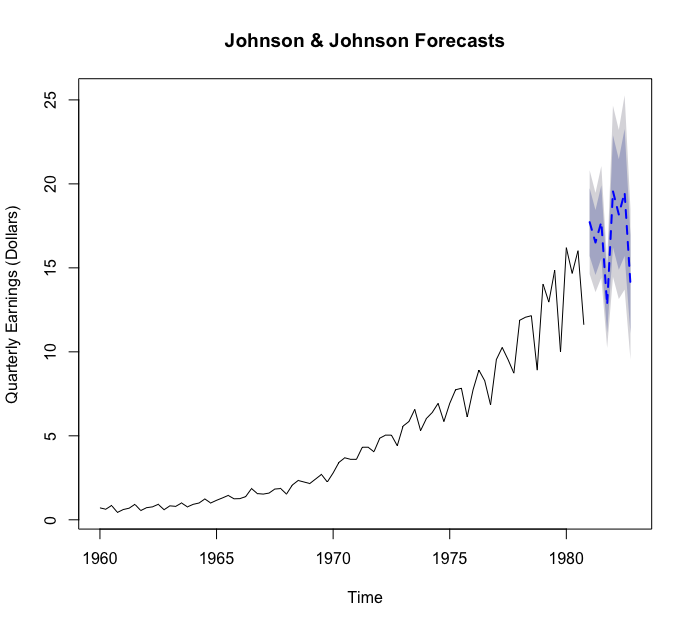
The selected model is one that has multiplicative trend, seasonal, and error components. The plot forecasts the next eight quarters. The forecasts are a dashed line, and the 80% and 95% confidence intervals are provided in light and dark gray, respectively.
As started earlier, exponential time-series modeling is popular because it can give good short-term forecasts in many situations. A second approach that is also popular is the Box-Jenkins methodology, commonly referred to as ARIMA models. These are described in the next blog.
Reference
[1] Robert I. Kabacoff. 2015. “Chapter 15 Time series” R IN ACTION Data analysis and graphics with R p 352-359
- Pexels, “night stars rotation starry sky”, pixabay.com. [Online]. Available: https://pixabay.com/photos/night-stars-rotation-starry-sky-1846734/