In this blog, I’ll introduce ARIMA forecasting models. In the autoregressive integrated moving average (ARIMA) approach to forecasting, predicted values are a linear function of recent actual values and recent errors of prediction (residuals). Before describing ARIMA models, we need to define a number of terms: lags, autocorrelation, partial autocorrelation, stationarity and differencing[1].
Prerequisite concepts
When you lag a time series, you shift it back by a given number of
observations. Autocorrelation measures the way observations in a time series
relate to each other.
is the correlation between a set of observations
(
) and
observationsk periods earlier
(
).
So
is the correlation between the Lag 1 and Lag 0 time series,
is the
correlation between the Lag 2 and Lag 0 time series, and so on. Plotting these
correlations produices an autocorrelation function (ACF) plot. The ACF plot is
used to select appropriate parameters for the ARIMA model and to assess the fit
of the final model. An ACF plot can be produced with the
acf() function in the
stats package or the Acf() function in the forecast package. Here, Acf()
function is used because it produces a plot that is somewhat easier to read.
A partial autocorrelation is the correlation between
and
with the effects of all Y values between the two removed. Partial
autocorrelations can also be plotted for multiple values of k. The PACF plot
can be generated with either the
pacf() function in the stats package or the
Pacf() function in the forecast package. The PACF plot is also used to
determine the most appropriate parameters for the ARIMA model.
ARIMA models are designed to fit stationary time series. In a stationary time
series, the statistical properties of the series don’t change over time. Because
stationary time series are assumed to have constant means, they can’t have a
trend component. Many non-stationary time series can be made stationary through
differencing. In differencing, each value of a time series
is replace with
.
Differencing a time series once removes a linear trend. Differencing it a second
time removes a quadratic trend. A third time removes a cubic trend. It’s rarely
necessary to difference more than twice.
Stationarity is often evaluated with a visuel inspection of a time-series plot. If the variance isn’t constant, the data are transformed. If there are trends, the data are difference. You can also use a statistical procedure called the Augmented Dickey-Fuller (ADF) test to evaluate the assumption of stationarity.
With these concepts in hand, we can turn to fitting models with an autoregressive (AR) component, a moving averages (MA) component, or both components (ARMA). Finally, we’ll examine ARIMA models that include ARMA components and differencing to achieve stationarity.
ARMA and ARIMA models
In an autoregressive model of order p, each value in a time series is predicted from a linear combinatioin of the previous p values
where
is a given value of the series, µ is the mean of the series, the
are the weights, and
is the irregular component.
In a moving average model of order q, each value in the time series is predicted from a linear combination of q previous errors. In this case
where the
are the errors of prediction and the
are the weights.
Combining the two approaches yields an ARMA(p, q) model of the form
that predicts each value of the time series from the past p values and q residuals.
An ARIMA(p, d, q) model is a model in which the time series has been differenced d times, and the resulting values are predicted from the previous p actual values and q previous errors. The predictions are “un-differenced” or integrated to achieve the final prediction.
Let’s apply each step in turn to fit an ARIMA model to the Nile time series.
Ensuring that the time series is stationary
First we plot the time series and assess its stationarity.

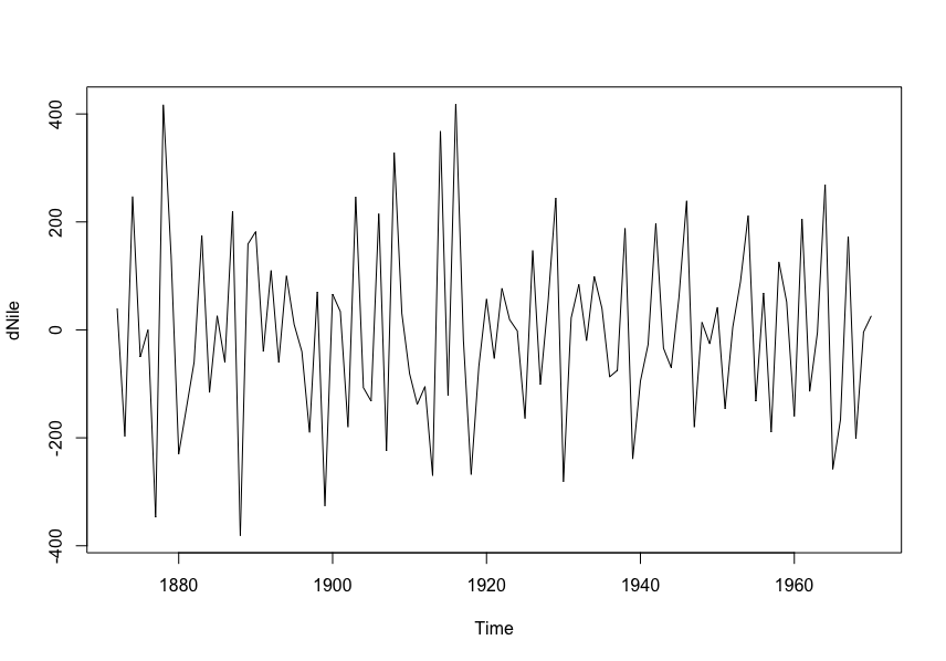
The variance appears to be stable across the years observed, so there’s no need
for a transformation. There may be a trend, which is supported by the results of
the ndiffs() function.
dNile <- diff(Nile)
plot(dNile)
adf.test(dNile)
The differenced time series is plotted as following and certainly looks more stationary. Applying the ADF test to the differenced series suggest that it’s now stationary, so we can proceed to the next step.
Identifying one or more reasonable models
Possible models are selected based on the ACF and PACF plots:
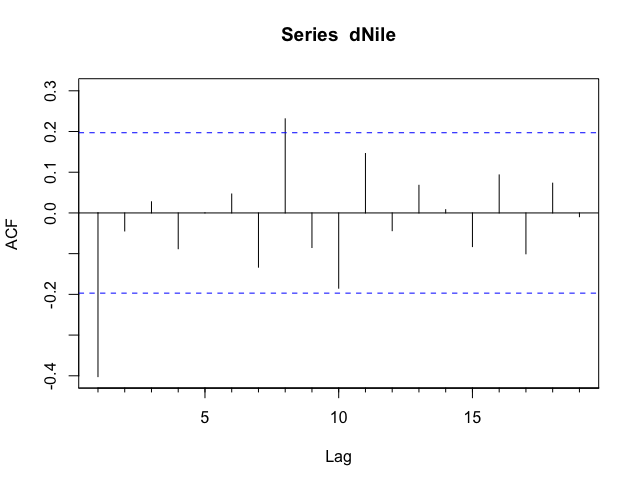
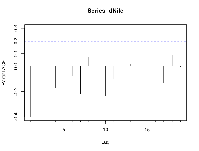
For the figure above, there appears to be one large autocorrelation at lag 1, and the partial autocorrelation trail off to zero as the lags get bigger. This suggests trying an ARIMA(0, 1, 1) model.
Fitting the model(s)
fit <- arima(Nile, order = c(0, 1, 1))
fit

# Call:
#   arima(x = Nile, order = c(0, 1, 1))
# Coefficients:
#   ma1
# -0.7329
# s.e.   0.1143
# sigma^2 estimated as 20600:  log likelihood = -632.55,  aic = 1269.09

accuracy(fit)
The coefficient for the moving averages (-0.73) is provided along with the AIC. If you fit other models, the AIC can help you choose which one is most reasonable. Smaller AIC values suggest better models. The accuracy measures can help you determine whether the model fits with sufficient accuracy.
Evaluating model fit
If the model is appropriate, the residuals should be normally distributed with mean zero, and the autocorrelations should be zero for every possible lag.
qqnorm(fit$residuals)
qqline(fit$residuals)
Box.test(fit$residuals, type = "Ljung-Box")
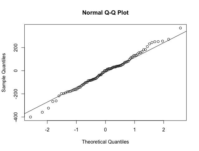
Normally distributed data should fall along the line. In this case, the results look good.
The Box.test() function provides a test that the autocorrelations are all zero.
The results suggest that the autocorrelations don’t differ from zero. This ARIMA
model appears to fit the data well.
Making forecasts
Once a final model has been chosen, it can be used to make predictions of future values.
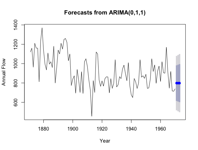
Point estimates are given by the blue dots, and 80% and 95% confidence bands are represented by dark and light bands, respectively.
In the last 3 blogs, we’ve looked at how to create time series in R, assess trends, and examine seasonal effects. Then we considered two of the most popular approaches to forecasting: exponential models and ARIMA models. Although these methodologies can be crucial in understanding and predicting a wide variety of phenomena, it’s important to remember that they each entail extrapolation - going beyond the data.
Reference
[1] Robert I. Kabacoff. 2015. “Chapter 15 Time series” R IN ACTION Data analysis and graphics with R p 359-366
- Pexels, “night stars rotation starry sky”, pixabay.com. [Online]. Available: https://pixabay.com/photos/night-stars-rotation-starry-sky-1846734/