I learnt Time Series from “R IN ACTION” in recent days and want to extract some important points for absorbing and summarizing the knowledge[1]. In this blog, I will simply introduce the methods for creating and manipulating time series, describing and plotting them, and decomposing them into level, trend, seasonal, and irregular (error) components.
Creating a time-series object in R
In order to work with a time series in R, you have to place it into a time-series object - an R structure that contains the observations, the starting and ending time of the series, and information about its periodicity. Once the data are in a time-series object, you can use numerous functions to manipulate, model, and plot the data.
A vector of numbers, or a column in a data frame, can be saved as a time-series
object using the ts() function.
Smoothing and seasonal decomposition
In this section, we’ll look at smoothing a time series to clarigy its general trend, and decomposing a time series in order to observe any seasonal effects.
Smoothing with simple moving averages
Time series typically have a significant irregular or error component. In order to discern any patterns in the data, you’ll frequently want to plot a smoothed curve that damps down these fluctuations. One of the simplest methods of smoothing a time series is to use simple moving averages.
Several functions in R can provide a simple moving average, including SMA()
in the TTR package, rollmean() in the zoo package, and ma() in the
forecast package.
Seasonal decomposition
Time-series data that have a seasonal aspect can be decomposed into a trend component, a seasonal component, and an irregular component. The trend component captures changes in level over time. The seasonal component captures cyclical effects due to the time of year. The irregular (of error) component captures thoses influences not described by the trend and seasonal effects.
The decomposition can be additive or multiplicative. In an additive model, the components sum to give the values of the times series. Specifically,
where the observation at time t is the sum of the contributions of the trend at time t, the seasonal effet at time t, and an irregular effect at time t.
In a multiplicative model, given by the equation
the trend, seasonal, and irregular influences are multiplied. Examples are given in the following figure[2].
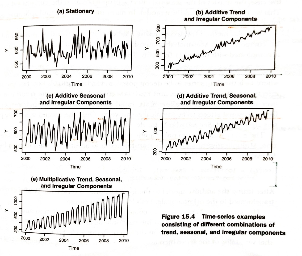
In the first plot (a), there is neither a trend nor a seasonal component. The only influence is a random fluctuation around a given level. In the second plot (b), there is an upward trend over time, as well as random fluctuations. In the third plot (c), there are seasonal effects and random fluctuations, but no overall trend away from a horizontal line. In the fourth plot (d), all three components are present: an upward trend, seasonal effects, and random fluctuations. You also see all three components in the final plot (e), but here they combine in a multiplicative way. Notice how the variability is proportional to the level: as the level increases, so does the variability. This amplification (or possible damping) based on the current level of the series strongly suggests a multiplicative model.
So far, we haven’t predicted any future values. In the next blog, we’ll consider the use of exponential models for forecasting beyond the available data.
Reference
[1] Robert I. Kabacoff. 2015. “Chapter 15 Time series” R IN ACTION Data analysis and graphics with R p 343-348
[2] Robert I. Kabacoff. 2015. “Chapter 15 Time series Figure 15.4” R IN ACTION Data analysis and graphics with R p 347
- Pexels, “night stars rotation starry sky”, pixabay.com. [Online]. Available: https://pixabay.com/photos/night-stars-rotation-starry-sky-1846734/