This blog reviews general methods for working with graphs. We’ll begin with how to create and save graphs, then talk about how to modify the features of graph.

Creating and saving graphs

Creating a new graph by issuing a high-level plotting command such as plot(), hist(), or boxplot() typically overwrites a previous graph. But how to create more than one graph and still have access to each? There are several methods.

First, we can open a new graph window before creating a new graph:

dev.new()
  statements to create graph 1
dev.new()
  statements to create graph 2

Each new graph will appear in the most recently opened window.

Then we can use the functions dev.new(), dev.next(), dev.prev(), dev.set() and dev.off() to have multiple graph window open at one time and choose which output is sent to which window. See help(dev.cur) for details.

If you want to save your graphs, you can do it via the following codes, sandwich the statements that produce the graph berween a statement that sets a destination and a statement that closes that destination.

pdf("my-graph.pdf")
  plot(mtcars$wt, mtcars$mpg)
  abline(lm(mtcars$mpg ~ mtcars$wt))
  title("Regression of MPG on Weight")
dev.off()

In additon to pdf(), we can use the functions win.metafile(), png(), jpeg(), bmp(), tiff(), xfig(), and postscript() to save graphs in other formats (Note: the win.metafile() function is only available on Windows platforms).

Graphical parameters

We can customize many features of a graph (fonts, colors, axes, and labels) through options called graphical parameters. One way to specify these options is through the par() function. Values set in this manner will be in effect for the rest of the session or until they’re changed, but not all high-level plotting functions allow us to specify all possible graphical parameters. The remainder of this blog will describe many important graphical parameters.

Symbols and lines

We can use graphical parameters to specify the plotting symbols and lines used in graphs. The relevant parameters are shown in the following table.

Table 1. Parameters for specifying symbols and lines

Parameter	Description
pch	Specifies the symbol to use when plotting points.
cex	Specifies the symbol size. 1 = default, 1.5 is 50% larger, 0.5 is 50% smaller, and so forth.
lty	Specifies the line type.
lwd	Specifies the line width. It's expressed relative to the default (1 = default). For example, 2 generates a line twice as wide as the default.

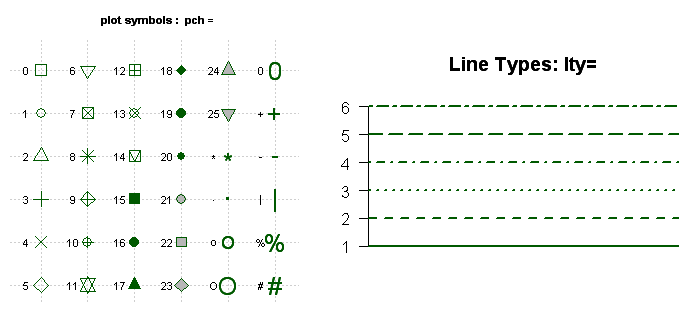
Plotting symbols specified with the pch parameter, line types specified with the lty parameter.

Colors

There are several color-related parameters in R. The following table shows some of the common ones.

Table 2. Parameters for specifying colors

Parameter	Description
col	Default plotting color.
col.axis	Color for axis text.
col.lab	Color for axis labels.
col.main	Color for titles.
col.sub	Color for subtitles.
fg	Color for the plot's foreground.
bg	Color for the plot's background.

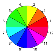
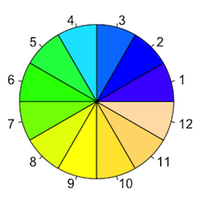
We can specify colors in R by index, name, hexadecimal, RGB, or HSV. For example, col = 1, col = "white", col = "#FFFFFF", col = rgb(1, 1, 1) and col = hsv(0, 0, 1) are equivalent ways of specifying the color white. The function colors() returns all avaiable color names. Moreover, R has a number of functions that can be used to create vectors of contiguous colors. These include rainbow(), heat.colors(), terrain.colors(), topo.colors() and cm.colors().

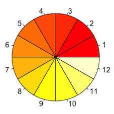
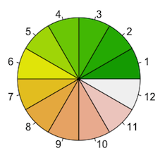
rainbow()	heat.colors()	terrain.colors()

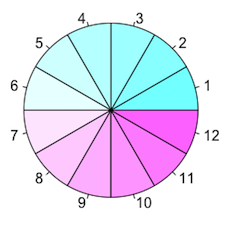
topo.colors()	cm.colors()

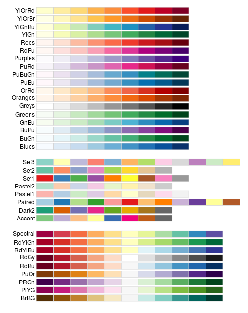
Furthermore, the RColorBrewer package is particularly popular for creating attractive color palettes, use the brewer.pal(n, name) function to generate a vector of colors. For the parameter name, all values are shown below.

Text characteristics

Graphic parameters are also used to specify text size, font, and style. Parameters controlling text size are explained in table 3. Font family and style can be controlled with font options (table 4).

Table 3. Parameters specifying text size

Parameter	Description
cex	Number indicating the amount by which plotted text should be scaled relative to the default. 1 = default, 1.5 is 50% larger, 0.5 is 50% smaller, and so forth.
cex.axis	Magnification of axis text relative to cex.
cex.lab	Magnification of axis labels relative to cex.
cex.main	Magnification of titles relative to cex.
cex.sub	Magnification of subtitles relative to cex.

Table 4. Parameters specifying font family, size, and style

Parameter	Description
font	Integer specifying the font to use for plotted text. 1 = plain, 2 = bold, 3 = italic, 4 = bold italic, and 5 = symbol (in Adobe symbol encoding).
font.axis	Font for axis text.
font.lab	Font for axis labels.
font.main	Font for titles.
font.sub	Font for subtitles.
ps	Font point size (roughly 1/72 inch). The text size = ps* cex.
family	Font family for drawing text. Standard values are serif, sans, and mono.

Graph and margin dimensions

Finally, we can control the plot dimensions and margin sizes using the parameters listed in table 5.

Table 5. Parameters specifying font family, size, and style

Parameter	Description
pin	Plot dimensions (width, height) in inches.
mai	Numerical vector indicating margin size, where c(bottom, left, top, right) is expressed in inches.
mar	Numerical vector indicating margin size, where c(bottom, left, top, right) is expressed in lines. The default is c(5, 4, 4, 2) + 0.1.

In the next blog, we’ll turn to the customization of text annotations, and look at ways to combine more than one graph into a single image.

Reference

• Steve Johnson, “art dirty texture brush”, www.pexels.com. [Online]. Available: https://www.pexels.com/photo/art-dirty-texture-brush-6868219/

PREVIOUSR: Working with GeoJSON data and resolve 'Error in ogrInfo'

NEXTR IN ACTION Review 3 - Time series (Part 1)