Thanks to DataCamp, I know more about Machine Learning. Among its different tasks, I first learnt an very important concept in supervised learning, Classification, which is suitable for the data with predefined classes. It automatically assign class to observations with features. Formally, an observation consists of a vector of features and a class. Classification model assigns automatically class with the input features, base on classes of previous ovservations. In this blog, I will talk about one algorithm of Classification: Decision Tree.
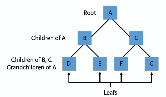
A decision tree is a decision support tool that uses a tree-like graph or model of decisions and their possible consequences. It is a flowchart-like structure in which each internal node represents a “test” on an attribute, each branch represents the outcome of the test and each leaf node represents a class label, the paths from root to leaf represents classification rules. Like the following structure:
Learn a decision tree
We should use training set to learn a decision tree; to do this, we need come up
with queries at each node. In order to realise recursive partitioning and
regression tree, we need to use the fonction rpart() in the library
rpart.
# For example, we use the "titanic" data frame (Source: Kaggle),
# which contains 714 observations and 4 variables: Survived,
# Pclass, Sex and Age.
# It has been divided into training and test sets (named train
# and test).
# Build a tree model: tree
tree <- rpart(Survived ~ ., train, method = "class")
# another expression
rpart(Survived ~ Pclass + Sex + Age, train, method = "class")
Then, we can use fonction fancyRpartPlot() to draw the decision tree.
fancyRpartPlot(tree)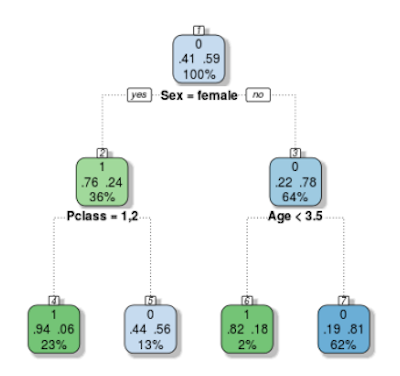
Let’s take the plot above as an example, which studies survivals in Titanic.The root node, at the top, shows 41% of passengers servive while 59% of them die. Next, if the passenger is a woman, we move to the left branch, then we see she has 76% probability to be alive. However, if she is in the second class, for the next step, we move to the right branch, which indicates she has only 44% probability to live. The rest can be done in the same manner.
Classify with the decision tree
The previous learning step involved proposing different tests on which to
split nodes and then to select the best tests using an appropriate splitting
criterion. You were spared from all the implementation hassles that come
with that: the rpart() function did all of that for you.
Now we are going to classify the instrances that are in the test set in the following steps:
- Use “tree” to predict the labels of the test set with the
predict()function - Create a confusion matrix of the predictions on the test set
- Use the confusion matrix to print out the accuracy
Following the previous codes, we can achieve the steps above the codes:
# Predict the values of the test set: pred
pred <- predict(tree, test, type = "class")

# Construct the confusion matrix: conf
conf <- table(test$Survived, pred)

# Print out the accuracy
sum( diag(conf) ) / sum(conf)  # 0.7990654
# Around 80% of all test instances have been classified correctly.
Pruning the tree
The number of nodes in the decision tree play an important role to see whether the decision tree will overfits to the training set or not. If you restrict the size of decision tree, the bias of resulting tree model will be higher, which will effectively decrease chance on overfit. This process is called Pruning the decision tree.
Now suppose that we will build a complex tree model: tree_cp. Then we can
use the prune() method to shrink the “tree_cp” to a more compact tree;
also specify the cp argument to be 0.01. As follows:
# Calculation of a complex tree
set.seed(1)
tree_cp <- rpart(Survived ~ ., train, method = "class",
           control = rpart.control(cp=0.00001))

# Draw the complex tree
fancyRpartPlot(tree_cp)

# Prune the tree: pruned
pruned <- prune(tree_cp, cp = 0.01)

# Draw pruned
fancyRpartPlot(pruned)
All things above are what I understand after learning from DataCamp, if you have some other ideas, don’t hesitate to tell me :)
Reference
- jplenio, “Tree nature wood sunset light”, pixabay.com. [Online]. Available: https://pixabay.com/photos/tree-nature-wood-sunset-light-3822149/