As I mentioned in my blog “What is Machine Learning”, Machine Learning tasks are typically classified into three broad categories, one of them is Supervised learning. In the supervised learning setting, it is important to understand the concept of two sets: Training set and Test set, which are useful to make good predictions about unseen observations.
When learning a predictive model, we should not use the complet dataset to train a model, we only use so-called training set for this; the other part of the dataset is called test set, which can be used to evaluate performance of model. It’s really important to realise that training set and test set are disjoint sets, they don’t have any observation in common, this makes it’s possible to test our model on unseen data.
Split the dataset
First, we need to split our dataset. Here I refer to DataCamp’s slide to explain its theorem. Suppose that we have N observations, K features and class labels for each observations y.
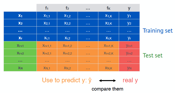
For the training set, we use the first r observations, then use the features and the class label to train a model. For the test set, we use the observations from r+1 until the end of the dataset, then use the features classified observations and compare the prediction with the actual class y. The confusion matrix that results gives us clear ideas of the actual predicted performance of the classifier.
Then, how to choose training set and test set? We should choose training set which is larger than test set, and the ratio is typically 3/1(arbitrary) in the training set over the test set. But make sure that your test set is NOT too small!
For example, you could use the following commands to shuffle a data frame df and divide it into training and test sets with a 60/40 split between the two.
n <- nrow(df)
shuffled_df <- df[sample(n), ]
train_indices <- 1:round(0.6 * n)
train <- shuffled_df[train_indices, ]
test_indices <- (round(0.6 * n) + 1):n
test <- shuffled_df[test_indices, ]
Distribution of the sets
It’s important that you choose wisely which elements you put in the training set and which ones you put in the test set. For Classification, the classes inside the training and test set must have similar distributions, avoid a class not being available in a set. For Classification & Regression, it’s always a smart idea to shuffle dataset before splitting.
Effect of sampling
Finally, be aware of the effect that the sampling of data in a certain way to compose the test set can influence the performance measures on the set. In order to add robustness to these measures, we can use cross-validation, which means that we use a learning algorithm to train a model multiple times, each time with different separations of training and test set. n-fold cross-validation means the test set is fold n times, each test set is 1/n size of total dataset.
For example, you will fold the dataset 6 times and calculate the accuracy for each fold. The mean of these accuracies forms a more robust estimation of the model’s true accuracy of predicting unseen data, because it is less dependent on the choice of training and test sets.
# Initialize the accs vector
accs <- rep(0,6)

for (i in 1:6) {
  # These indices indicate the interval of the test set
   indices <- (((i-1) * round((1/6)*nrow(shuffled))) + 1)
                    :((i*round((1/6) * nrow(shuffled))))
  # Exclude them from the train set
  train <- shuffled[-indices,]

  # Include them in the test set
  test <- shuffled[indices,]

  # A model is learned using each training set
  tree <- rpart(Survived ~ ., train, method = "class")

  # Make a prediction on the test set using tree
  pred <- predict(tree, test, type = "class")

  # Assign the confusion matrix to conf
  conf <- table(test$Survived, pred)

  # Assign the accuracy of this model to the ith index in accs
  accs[i] <- sum(diag(conf))/sum(conf)
}
Reference
- Kendal, “person holding amber glass bottles”, unsplash.com. [Online]. Available: https://unsplash.com/photos/L4iKccAChOc