In this blog, I will talk about some basic elements for creating a graph/graphs by package matplotlib.pyplot.

Figures & Axes & Axis

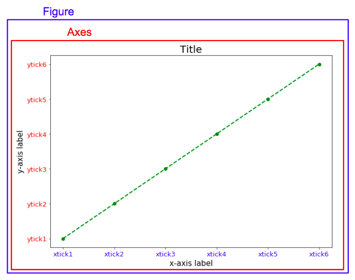
The figure can be seen as the canvas, on which all drawing components are plotted. The figure consists of axes, which are subdivisions of the figure. Each of the axes consists of one or more axis (horizontal (x-axis), vertical (y-axis) or even depth (z-axis))[source].

import matplotlib.pyplot as plt
import numpy as np

data = np.arange(6)
plt.figure(figsize=(10, 7))
plt.plot(data, color='green', marker='.',
         linestyle='--', linewidth=2, markersize=12)
         
plt.title('Title', loc='center', fontdict={'fontsize': 20})
plt.xticks(np.arange(6),
           ('xtick1', 'xtick2', 'xtick3',
            'xtick4', 'xtick5', 'xtick6'))
plt.yticks(np.arange(6),
           ('ytick1', 'ytick2', 'ytick3',
            'ytick4', 'ytick5', 'ytick6'))
plt.tick_params(axis='x', labelsize=13, colors='b')
plt.tick_params(axis='y', labelsize=13, colors='r')
plt.xlabel('x-axis label', fontdict={'fontsize': 15})
plt.ylabel('y-axis label', fontdict={'fontsize': 15})

plt.show()

Detail

plt.figure(figsize=(10, 7))

Parameter figsize in function plt.figure() places a tuple of integers (width, height in inches)

plt.plot(data, color='green', marker='.',
         linestyle='--', linewidth=2, markersize=12)

Function plt.plot() creates a figure, data shows the horizontal/vertical coordinates of the data points, marker and linestyle specify the marker style for each point and line style between each two points.

plt.title('Title', loc='center', fontdict={'fontsize': 20})

plt.title() helps us to add a title for the figure, and put it on the left, middle or right by loc parameter, fontdict is a dictionary controlling the appearance of the title text.

plt.xticks(np.arange(6),
           ('xtick1', 'xtick2', 'xtick3',
            'xtick4', 'xtick5', 'xtick6'))
plt.yticks(np.arange(6),
           ('ytick1', 'ytick2', 'ytick3',
            'ytick4', 'ytick5', 'ytick6'))

plt.xticks() and plt.yticks() get or set the current tick locations and labels of the x-axis/y-axis. The first parameter locs is a list of positions at which ticks should be placed, the second parameter labels, which is optional, is a list of explicit labels to place at the given locs. If your data is in a pandas dataframe, you can use df.index to specify locs and use df.col1 to specify labels.

plt.tick_params(axis='x', labelsize=13, colors='b')
plt.tick_params(axis='y', labelsize=13, colors='r')

plt.tick_params() changes the appearance of ticks, tick labels, and gridlines. Parameter axis specifies which axis to apply the parameters to, labelsize changes tick label font size in points or as a string (e.g., ‘large’), colors changes the tick color and the label color to the same value: mpl color spec.

plt.xlabel('x-axis label', fontdict={'fontsize': 15})
plt.ylabel('y-axis label', fontdict={'fontsize': 15})

plt.xlabel() and plt.ylabel() set the x-axis/y-axis label of the current axes. First parameter label describe label of x-axis or y-axis, fontdict is a dictionary controlling the appearance of the label, here I set the label font size to be 15.

Subplots

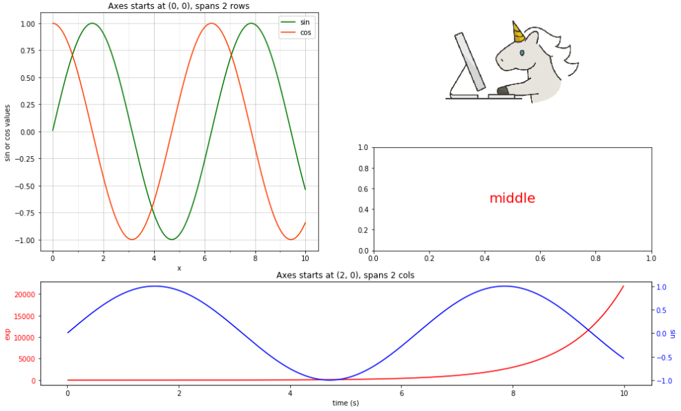
A figure can contain a set of subplots.

import matplotlib.cbook as cbook
import matplotlib.pyplot as plt
import numpy as np

x = np.arange(0.01, 10.0, 0.01)
y1 = np.sin(x)
y2 = np.cos(x)
y3 = np.exp(x)

fig, axarr = plt.subplots(nrows=3, ncols=2, figsize=(16, 10))

ax00 = plt.subplot2grid((3, 2), (0, 0), rowspan=2)
ax00.set_title('Axes starts at (0, 0), spans 2 rows',
               fontdict={'fontsize': 12})
ax00.plot(x, y1, label='sin', color='green')
ax00.plot(x, y2, label='cos', color='orangered')

ax00.set_xticks(np.arange(11), minor=True)
ax00.grid(which='major', alpha=0.5)
ax00.grid(which='minor', alpha=0.2)
ax00.set_xlabel('x')
ax00.set_ylabel('sin or cos values')
ax00.legend()

ax20 = plt.subplot2grid((3, 2), (2, 0), colspan=2)
ax20.set_title('Axes starts at (2, 0), spans 2 cols',
               fontdict={'fontsize': 12})

ax20.plot(x, y3, color='r')
ax20.set_xlabel('time (s)')
ax20.set_ylabel('exp', color='r')
ax20.tick_params(axis='y', labelcolor='r')

ax20_2 = ax20.twinx()
ax20_2.plot(x, y1, color='b')
ax20_2.set_ylabel('sin', rotation=270, color='b')
ax20_2.tick_params(axis='y', labelcolor='b')

ax01 = axarr[0, 1]
image_file = cbook.get_sample_data('images/20180526-unicorn.png')
image = plt.imread(image_file)
ax01.imshow(image)
ax01.axis('off')

ax11 = axarr[1, 1]
ax11.text(0.5, 0.5, 'middle',
          horizontalalignment='center',
          verticalalignment='center',
          fontsize=20, color='red',
          transform=ax11.transAxes)

plt.subplots_adjust(hspace=0.3)
plt.show()

Detail

fig, axarr = plt.subplots(nrows=3, ncols=2, figsize=(16, 10))

Function plt.subplots() creates a figure and a set of subplots, this utility wrapper makes it convenient to create common layouts of subplots, including the enclosing figure object, in a single call.

ax00 = plt.subplot2grid((3, 2), (0, 0), rowspan=2)

subplot2grid() creates an axis at specific location inside a regular grid, the first subplot on the left spans 2 rows and the subplot at the bottom spans 2 columns. First parameter shape is a sequence of 2 integers, it is the shape of grid in which to place axis, first entry is number of rows, second entry is number of columns. loc is also a sequence of 2 ints, which describes location to place axis within grid, first entry is row number, second entry is column number. rowspan and colspan is a integer, they are the number of rows/columns for the axis to span to the right/downwards.

ax00.set_xticks(np.arange(11), minor=True)

set_xticks() helps to set the x ticks with list of ticks for a subplot, similar as plt.xticks(), first parameter ticks is a list of x-axis tick locations; if minor=False sets major ticks, if True sets minor ticks.

ax00.grid(which='major', alpha=0.5)
ax00.grid(which='minor', alpha=0.2)

plt.grid() sets the axes grids on or off, which can be ‘major’ (default), ‘minor’, or ‘both’ to control whether major tick grids, minor tick grids, or both are affected, alpha specifies the transparency of the grid (float, 0.0 transparent through 1.0 opaque). You can also fill parameter axis to control which set of gridlines are drawn.

ax00.legend()

legend() places a legend on the axes. When you do not pass in any extra arguments, the elements to be added to the legend are automatically determined. To make a legend for lines which already exist on the axes, simply call this function with an iterable of strings, one for each legend item. For full control of which artists have a legend entry, you can pass an iterable of legend artists followed by an iterable of legend labels respectively.

ax20_2 = ax20.twinx()

You might find that in the bottom plot, there are two different axes that share the same x axis (more details). Function axes.twinx() helps us to make a second axes that shares the x-axis. The new axes will overlay ax (or the current axes if ax is None). The ticks for ax2 will be placed on the right, and the ax2 instance is returned.

ax11 = axarr[1, 1]

If we don’t need to span rows/columns, like the plot on the right side, we only need to specify the location of the graph with [row, column], so here with axarr[1, 1].

ax11.text(0.5, 0.5, 'middle',
          horizontalalignment='center',
          verticalalignment='center',
          fontsize=20, color='red',
          transform=ax11.transAxes)

Function plt.text() can add text to the axes. First two parameters x and y are scalars, they show the position to place the text. Third parameter s is the text string. horizontalalignment and verticalalignment set the horizontal and verticalalignment to one of left/center/right.

image_file = cbook.get_sample_data('images/20180526-unicorn.png')
image = plt.imread(image_file)
ax01.imshow(image)
ax01.axis('off')

At the right top corner, I put an image of unicorn (source) with plt.imshow(), and hide the axis with axes.axis('off'). Package cbook is a collection of utility functions and classes, one of its function get_sample_data() returns a sample data file, the first parameter fname is a path relative to the mpl-data/sample_data directory. plt.imread() reads an image from a file into an array, fname may be a string path, a valid URL, or a Python file-like object. If using a file object, it must be opened in binary mode. plt.imshow() displays an image on the axes.

plt.subplots_adjust(hspace=0.3)

plt.subplots_adjust() helps us to adjust the subplot layout, I increased a little the height between subplots with parameter hspace.

Reference

• Steve Johnson, “painting wallpaper”, www.pexels.com. [Online]. Available: https://www.pexels.com/photo/painting-wallpaper-1070527/

PREVIOUSIntroduction to pandas data structures

NEXTMatplotlib Series 1: Bar chart