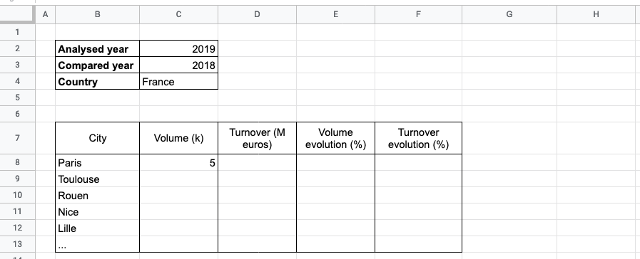
During my work, sometimes I need to create a dynamic Excel workbook for clients. The screenshot below is a simple example, we can filter “analysed year”, “compared year” and “country” to get some KPIs of selected country on selected year.
How can we look for a value with multiple conditions? In this blog, I’ll
show you how to accomplish it with functions vlookup or index & match with
following points:
- Usage
- Example
- Pro & cons
VLOOKUP function
Usage
Use VLOOKUP when you need to find things in a table or a range by row. For
example, look up the price of an automotive part by the part number, or find an
employee name based on their employee ID.
Syntax
VLOOKUP (lookup_value, table_array, col_index_num, [range_lookup])
lookup_value: (required) The value you want to look up. The value you want to look up must be in the first column of the range of cells you specify in thetable_arrayargument.table_array: (required) The range of cells in which theVLOOKUPwill search for thelookup_valueand the return value.col_index_num: (required) The column number (starting with 1 for the left-most column oftable_array) that contains the return value.range_lookup: (optional) A logical value that specifies whether you wantVLOOKUPto find an approximate or an exact match: Approximate match - 1/TRUE, Exact match - 0/FALSE.
Example
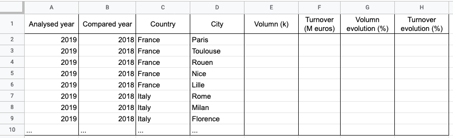
Now back to the use case at the beginning of the blog, how can we get Paris’ “volume(k)” in 2019 vs. 2018 with the following worksheet?
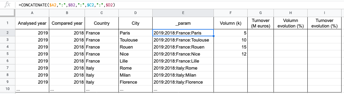
Considering there are multiple values to look up, and the lookup_value can
only be one column, so what we can do is concatenating columns “Analysed year”,
“Compared year”, “Country” and “City” into a new column named “_param” with
CONCATENATE function.
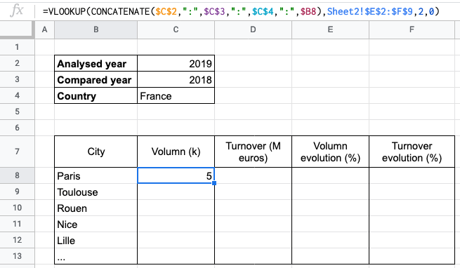
Then we can get the result with vlookup as following:
Pro & cons
vlookup is efficacy and easy to use, since it looks for value only in one
column and search its result in one column as well, but if you want to look for
multiple values like the example, you need to concatenate them as the
“lookup_value” firstly, then apply the vlookup function.
INDEX + MATCH function
Usage
INDEX function
The INDEX function returns a value or the reference to a value from within a
table or range. Here I will mainly talk about the case when you want to return
the value of a specified cell or array of cells (so-called Array form), if you
want to return a reference to specified cells, see Reference form.
Returns the value of an element in a table or an array, selected by the row and column number indexes. Use the array form if the first argument to INDEX is an array constant.
Syntax
INDEX(array, row_num, [column_num])
array: (required) A range of cells or an array constant.- If the array contains only one row or column, the corresponding
row_numorcolumn_numargument is optional. - If the array has more than one row and more than one column, and only
row_numorcolumn_numis used,INDEXreturns an array of the entire row or column in the array.
- If the array contains only one row or column, the corresponding
row_num: (required) Unlesscolumn_numis present. Selects the row in the array from which to return a value. Ifrow_numis omitted,column_numis required.column_num: (optional) Selects the column in the array from which to return a value. Ifcolumn_numis omitted,row_numis required.
MATCH function
The MATCH function searches for a specified item in a range of cells, and then
returns the relative position of that item in the range. For example, if the
range A1:A3 contains the values 5, 25, and 38, then the formula
=MATCH(25,A1:A3,0) returns the number 2, because 25 is the second item in the
range.
Syntax
MATCH(lookup_value, lookup_array, [match_type])
lookup_value: (required) The value that you want to match inlookup_array. Thelookup_valueargument can be a value (number, text, or logical value) or a cell reference to a number, text, or logical value.lookup_array: (required) The range of cells being searched.match_type: (optional) The number -1, 0, or 1. Thematch_typeargument specifies how Excel matcheslookup_valuewith values inlookup_array. The default value for this argument is 1.- 1 or omitted:
MATCHfinds the largest value that is less than or equal tolookup_value. - 0:
MATCHfinds the first value that is exactly equal tolookup_value. - -1:
MATCHfinds the smallest value that is greater than or equal tolookup_value.
- 1 or omitted:
Example
Same as above, let’s back to the use case at the beginning of the blog, how can we get Paris’ “volume(k)” in 2019 vs. 2018 with the following worksheet?
Then we can get the result with index & match as following:
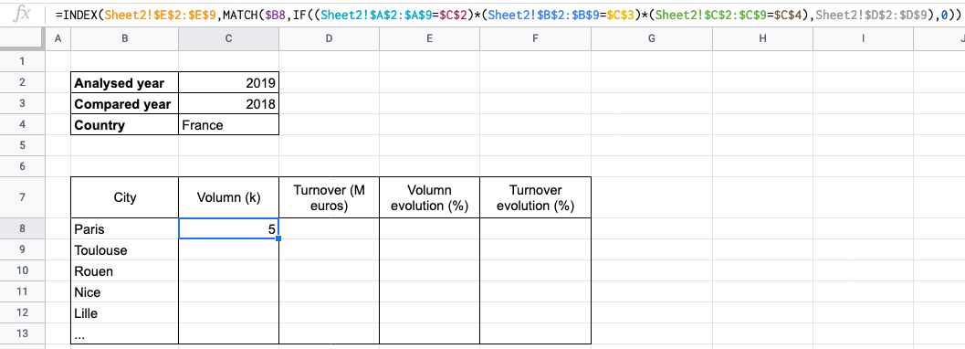
We can use INDEX to help us get the result, so we set the volume’s column of
sheet2 as array, set “0” as column_num, it remains row_num to set. In
order to find out the row_num, we need the help of MATCH. First, we set one
of “Analysed year”, “Compared year”, “Country” and “City” as the lookup_value,
here I take “City”, then set the ranges which is equal to each other conditions
as lookup_array, and find the first value that is exactly equal to
lookup_value.
Pro & cons
Inverse to the negative points of vlookup, we don’t need to concatenate all
conditions into one column, we can intersect different conditions as many as you
want with MATCH, but the cost is it might take a long time to find the final
result.
Conclusion
In this blog, I presented 3 excel functions, vlookup, index, and match, on
their usages, syntaxes, applied them in different use cases, and their pro & cons.
Hope it’s useful for you!
Reference
- “VLOOKUP function”, support.microsoft.com. [Online]. Available: https://support.microsoft.com/en-us/office/vlookup-function-0bbc8083-26fe-4963-8ab8-93a18ad188a1
- “INDEX function”, support.microsoft.com. [Online]. Available: https://support.microsoft.com/en-us/office/index-function-a5dcf0dd-996d-40a4-a822-b56b061328bd
- “MATCH function”, support.microsoft.com. [Online]. Available: https://support.microsoft.com/en-us/office/match-function-e8dffd45-c762-47d6-bf89-533f4a37673a
- “CONCATENATE function”, support.microsoft.com. [Online]. Available: https://support.microsoft.com/en-us/office/concatenate-function-8f8ae884-2ca8-4f7a-b093-75d702bea31d
- Siam Hasan Khan, “Match Two Columns in Excel and Return a Third (3 Ways)”, www.exceldemy.com. [Online]. Available: https://www.exceldemy.com/match-two-columns-in-excel-and-return-a-third/
- Denys Nevozhai, “Road, HD City Wallpapers, Intersection”, unsplash.com. [Online]. Available: https://unsplash.com/photos/7nrsVjvALnA