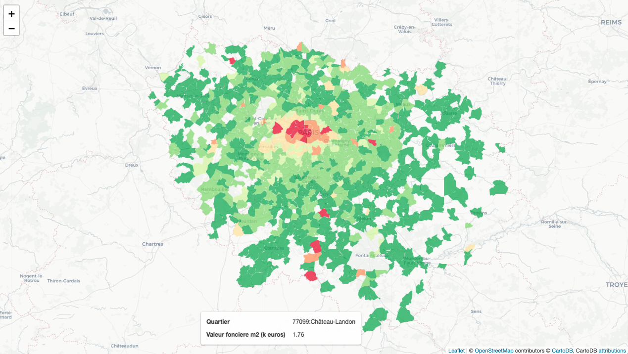
A map can clearly present information in terms of geography. Recently I learnt
how to realize geovisualization with folium module in Python. In this blog, I
will talk about how to draw a map like the one above with folium with the
following points:
- Data preparation
- Geovisualization with
folium
Data preparation
Import datasets
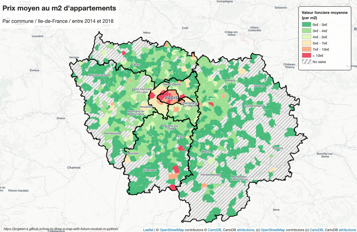
The map above describes the apartments’ average price per m2 of Ile-de-France, between 2014 and 2018. Before all, we need sold apartments’ data for calculating average price per m2, need communities’ and departments’ polygon data to draw areas on the map.
vf = pd.read_csv('idf.1418.csv')
dept_geo = geopandas.read_file('departements.geojson', driver='GeoJSON')
communesidf_geo = geopandas.read_file('Communes_IDF.json', driver='JSON')
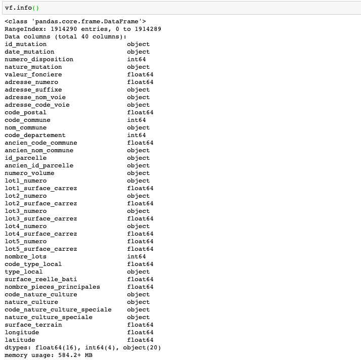
In the sold apartments’ dataset, we have data like “id_mutation” to identify the transaction, “nature_mutation” specifies the sale’s nature, “valeur_fonciere” presents the sold price, “code_commune”, “nom_commune” and “code_departement” specify the communities and departments, “surface_reelle_bati” describes the real surface area, longitude and latitude can help us to determine the location.
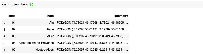
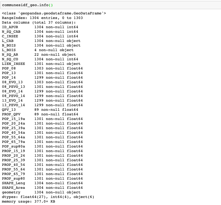
For the polygon data, we only need “code” and “C_INSEE” to match the department and community and “geometry” to draw polygons.
Data cleaning
Now we have sold apartments and polygon data for the whole France, what we need is the data that relative to Ile-de-France:
departments = {'75', '77', '78', '91', '92', '93', '94', '95'}
dept_geo = dept_geo[dept_geo['code'].isin(departments)]

vf = vf[(vf['type_local'] == 'Appartement') &
        (vf['nature_mutation'] == 'Vente') &
        (vf['valeur_fonciere'] > 0) &
        (vf['surface_reelle_bati'] > 0) &
        (vf['longitude'].isnull() == False) &
        (vf['latitude'].isnull() == False) &
        ((vf['lot1_surface_carrez'].isnull() == False) |
         (vf['lot2_surface_carrez'].isnull() == False) |
         (vf['lot3_surface_carrez'].isnull() == False) |
         (vf['lot4_surface_carrez'].isnull() == False) |
         (vf['lot5_surface_carrez'].isnull() == False) )]
Then we use “valeur_fonciere” and surface to calculate average price per m2 for each community with the following function:
def calculate_vf_m2(nature_culture, valeur_fonciere,
                    surface_terrain, surface_reelle_bati):
    if math.isnan(surface_terrain) == False and nature_culture in ['sols', 'jardins', "terrains d'agrément"]:
        return valeur_fonciere / surface_terrain
    else:
        return valeur_fonciere / surface_reelle_bati
When the sold nature is “sols”, “jardins” or “terrains d’agrément”, the sold surface area is indicated as “surface_terrain”, so the price per m2 is obtained by dividing “valeur_fonciere” by “surface_terrain”; otherwise, divide “valeur_fonciere” by “surface_reelle_bati”.
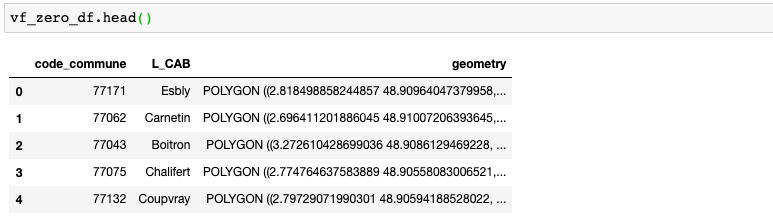
The last 2 steps before drawing the map are transform the coordinates to
geopoints with shapely.geometry.Point(), match each polygon to community,
and find out which communities(polygons) have no sales.
vf['points'] = vf.apply(lambda row: Point(row['longitude'],
row['latitude']),
axis='columns')
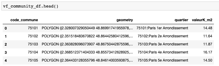
vf_zero = communesidf_geo[communesidf_geo['code_commune'].isin(vf['code_commune'].unique())==False]Now, we have 2 dataframes vf_community_df and vf_zero_df to display average
price per m2 for each community.
Geovisualization with “folium”
In this part, I’ll complete the map with the following elements:
- Colormap
- Map base
- Sold apartments layer
- No-sales layer
- Department layer
- Add customized title and legend
Colormap
import branca.colormap as cm

colormap_dept = cm.StepColormap(
    colors=['#00ae53', '#86dc76', '#daf8aa',
            '#ffe6a4', '#ff9a61', '#ee0028'],
    vmin=min(vf_community_df['valeurK_m2']),
    vmax=max(vf_community_df['valeurK_m2']),
    index=[0, 3, 4, 5, 7, 10, 25])
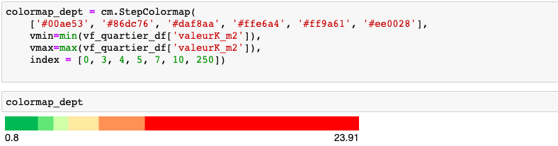
branca.colormap.StepColormap creates a ColorMap based on linear interpolation
of a set of colors over a given index. index presents the values
corresponding to each color, it has to be sorted, and have the same length as
colors; if None, a regular grid between vmin and vmax is created.
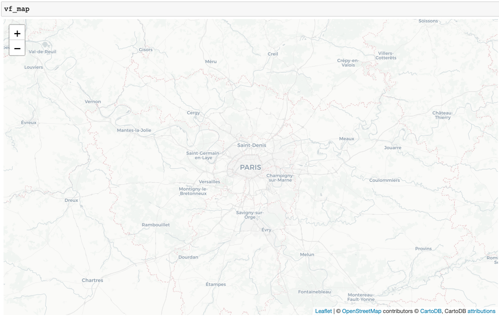
Map base
import folium
vf_map = folium.Map(location=[48.856614, 2.3522219],
                    zoom_start = 9, tiles='cartodbpositron')
Sold apartments layer
style_function = lambda x: {
    'fillColor': colormap_dept(x['properties']['valeurK_m2']),
    'color': '',
    'weight': 0.0001,
    'fillOpacity': 0.7
}

folium.GeoJson(
    vf_community_df,
    style_function=style_function,
    tooltip=folium.GeoJsonTooltip(
        fields=['quartier', 'valeurK_m2'],
        aliases=['Quartier', 'Valeur fonciere m2 (k euros)'],
        localize=False
    ),
    name='Community').add_to(vf_map)
I created the style_function to assign community-color in terms of
“valeurK_m2”, set color as '' since the default color for border is blue,
but in my case I don’t need color. Furthermore, I used folium.GeoJsonTooltip
to add the popup.
No-sales layer
from folium import plugins

def style_zero_function(feature):
    default_style = {
        'fillOpacity': 0.03,
        'color': 'gray',
        'weight': 0.0001
    }

    default_style['fillPattern'] = plugins.pattern.StripePattern(angle=-45)

    return default_style

folium.GeoJson(
    vf_zero_df,
    style_function=style_zero_function,
    tooltip=folium.GeoJsonTooltip(
        fields=['code_commune'],
        aliases=['Code commune'],
        localize=False
    ),
    name='Community').add_to(vf_map)
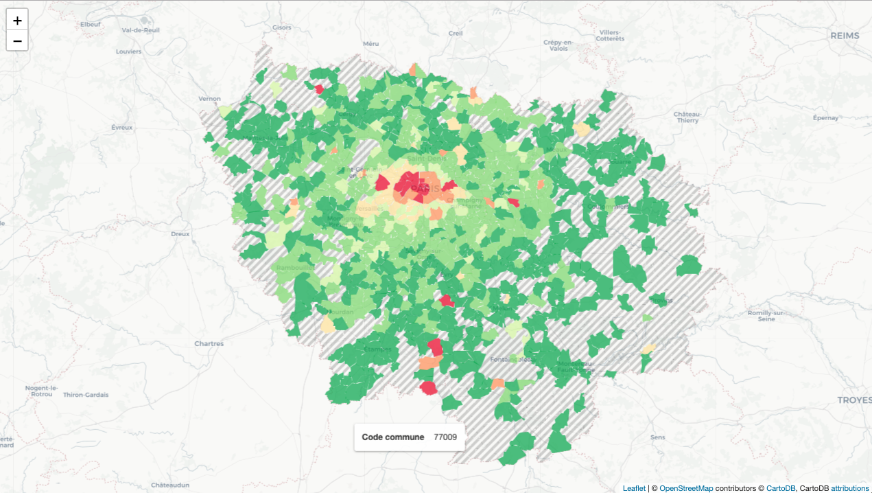
Before creating a new layer, I created style_zero_function to specify
no-sales communities’ pattern. For creating a new layer, it’s the same as the
first layer.
Department layer
folium.GeoJson(
    dept_geo,
    style_function = lambda x: {
        'color': 'black',
        'weight': 2.5,
        'fillOpacity': 0
    },
    name='Departement').add_to(vf_map)
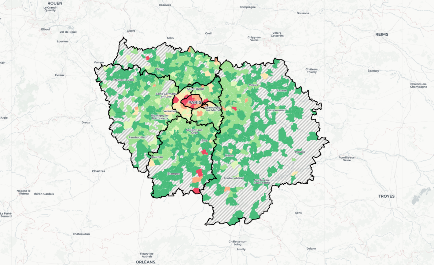
This step is to add border for each department, so we don’t need fillcolor.
Add customized title and legend
<div id='maplegend' class='maplegend'
    style='position: absolute; z-index:9999; border:0px; background-color:rgba(255, 255, 255, 0.8);
     border-radius:6px; padding: 10px; font-size:25px; left: 0px; top: 0px;'>

<div class='legend-title'>Prix moyen au m2 d'appartements</div>
<div class='legend-scale'><font size="3">Par commune / Ile-de-France / entre 2014 et 2018</font></div>
</div>
Inspired by this example, I customized title for the map, for
more details, you can find it here. To customizing the colormap
legend, you only need to replace legend-title and legend-scale by the
following codes:
<div id='maplegend' class='maplegend'
    style='position: absolute; z-index:9999; border:2px solid grey; background-color:rgba(255, 255, 255, 0.8);
     border-radius:6px; padding: 10px; font-size:14px; right: 20px; top: 20px;'>

<div class='legend-title'>Valeur fonciere moyenne<br>(par m2)</div>
<div class='legend-scale'>
  <ul class='legend-labels'>
    <li><span style='background:#00ae53;opacity:0.7;'></span>0k€ - 3k€</li>
    <li><span style='background:#86dc76;opacity:0.7;'></span>3k€ - 4k€</li>
    <li><span style='background:#daf8aa;opacity:0.7;'></span>4k€ - 5k€</li>
    <li><span style='background:#ffe6a4;opacity:0.7;'></span>5k€ - 7k€</li>
    <li><span style='background:#ff9a61;opacity:0.7;'></span>7k€ - 10k€</li>
    <li><span style='background:#ee0028;opacity:0.7;'></span>> 10k€</li>
    <li><span style='background:repeating-linear-gradient(
    -55deg,
    #ffffff,
    #ffffff 5px,
    #b2b2b2 5px,
    #b2b2b2 10px);
    opacity:0.7;'></span>No sales</li>
  </ul>
</div>
</div>
Reference
- DGFiP, “Demandes de valeurs foncières géolocalisées”, data.gouv.fr. [Online]. Available: https://www.data.gouv.fr/fr/datasets/demandes-de-valeurs-foncieres-geolocalisees/
- Grégoire David, “Departments polygon”, github.com. [Online]. Available: https://github.com/gregoiredavid/france-geojson/blob/master/departements.geojson
- APUR, “APUR : Communes - Ile de France”, data.gouv.fr. [Online]. Available: https://www.data.gouv.fr/fr/datasets/apur-communes-ile-de-france/
- branca, “branca.colormap”, python-visualization.github.io/branca. [Online]. Available: https://python-visualization.github.io/branca/colormap.html#
- folium, “Preleminary demo of the pattern plugin for Folium”, nbviewer.jupyter.org. [Online]. Available: https://nbviewer.jupyter.org/github/python-visualization/folium/blob/master/examples/plugin-patterns.ipynb
- “How does one add a legend (categorical) to a folium map”, nbviewer.jupyter.org. [Online]. Available: https://nbviewer.jupyter.org/gist/talbertc-usgs/18f8901fc98f109f2b71156cf3ac81cd
- WikiImages, “Earth map summer July continents”, pixabay.com_. [Online]. Available: https://pixabay.com/photos/earth-map-summer-july-continents-11048/