Have your heard about the classic use case of association analysis - “Beer and diaper” at Walmart? In this story, Walmart found that beer and diapers were often sold together, we can use association analysis to explain this image.
In this blog, I will introduce some useful concepts and then a use case of association analysis.
Useful Concepts (resource: Wikipedia)
Association analysis is a rule-based machine learning method for discovering interesting relations between variables in large databases. It is intended to identify strong rules discovered in databases using some measures of interestingness.
Let X be an itemset, X => Y an association rule and T a set of transactions of a given database.
Support
Support is an indication of how frequently the itemset appears in the dataset. The support of X with respect to T is defined as the proportion of transactions t in the dataset which contains the itemset X.
Confidence
Confidence is an indication of how often the rule has been found to be true.
The confidence value of a rule, X => Y, with respect to a set of transactions T, is the proportion of the transactions that contains X which also contains Y.
Confidence is defined as:
Note that
means the support of the union of the items in X and Y. This is somewhat
confusing since we normally think in terms of probabilities of events and not
sets of items. We can rewrite
as the probability
,
where
and
are the events that a transaction contains itemset X and Y,
respectively.
Thus confidence can be interpreted as an estimate of the conditional probability
,
the probability of finding the RHS of the rule in transactions under the
condition that these transactions also contain the LHS.
Lift
The lift of a rule is defined as:
or the ratio of the observed support to that expected if X and Y were independent.
If the rule had a lift of 1, it would imply that the probability of occurrence of the antecedent and that of the consequent are independent of each other. When two events are independent of each other, no rule can be drawn involving those two events.
If the lift is > 1, that lets us know the degree to which those two occurrences are dependent on one another, and makes those rules potentially useful for predicting the consequent in future data sets.
The value of lift is that it considers both the confidence of the rule and the overall data set.
Use case
Dataset
I will use the Groceries dataset which comes from package arules.
library(arules)

data(Groceries)

class(Groceries)
[1] "transactions"
attr(,"package")
[1] "arules"

inspect(head(Groceries, 3))
    items
[1] {citrus fruit,semi-finished bread,margarine,ready soups}
[2] {tropical fruit,yogurt,coffee}
[3] {whole milk}

summary(Groceries)
transactions as itemMatrix in sparse format with
 9835 rows (elements/itemsets/transactions) and
 169 columns (items) and a density of 0.02609146

most frequent items:
 whole milk other vegetables  rolls/buns  soda  yogurt  (Other)
       2513             1903       1809   1715    1372    34055

element (itemset/transaction) length distribution:
sizes
   1    2    3    4    5    6    7    8    9   10   11   12   13
2159 1643 1299 1005  855  645  545  438  350  246  182  117   78
  14   15   16   17   18   19   20   21   22   23   24   26   27
  77   55   46   29   14   14    9   11    4    6    1    1    1
  28   29   32
   1    3    1

   Min. 1st Qu.  Median    Mean 3rd Qu.    Max.
  1.000   2.000   3.000   4.409   6.000  32.000

includes extended item information - examples:
       labels  level2           level1
1 frankfurter sausage meat and sausage
2     sausage sausage meat and sausage
3  liver loaf sausage meat and sausage
Before creating the model, we have a view of data. In this dataset, there are 9835 transactions and 169 items, the density of 1 in sparse matrix is 0.02609146. The 5 most frequent items are whole milk, other vegetables, rolls/buns, soda and yogurt. Element length distribution shows items’ amount in the transaction and transactions’ amount. For instance, 2159 transactions have only 1 item, 545 transactions have 7 items, and only 1 transaction has 27 items.
Model
The value of support is useful for creating the model. We can use the function
itemFrequencyPlot() to check top N frequent item.
itemFrequencyPlot(Groceries, topN=10, type="absolute", main="Item Frequency")
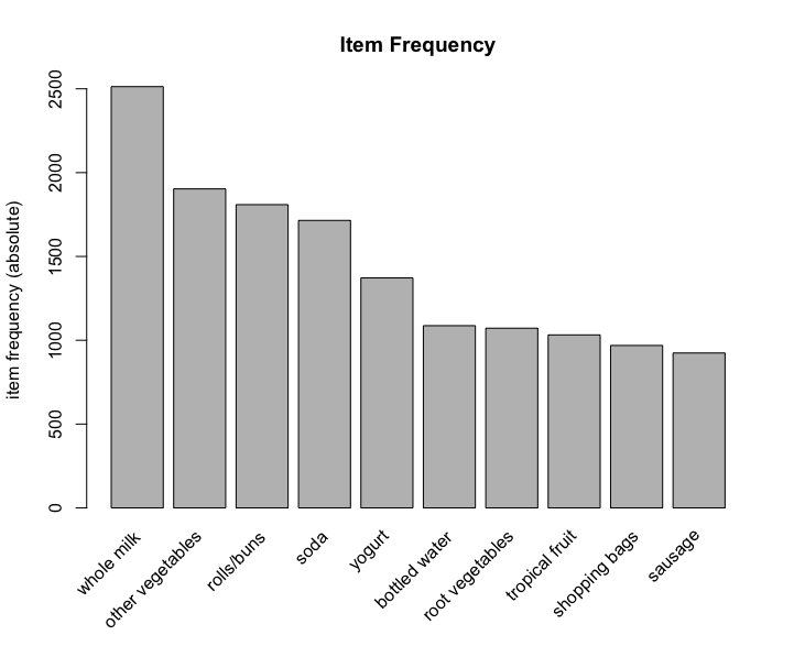
Now we have a clear idea about the data, next we can create the model.
rules <- apriori (Groceries, parameter = list(supp = 0.001, conf = 0.5))

rulesLift <- sort (rules, by = "lift", decreasing = T)
inspect(head(rulesLift))
    lhs                                                  rhs              support     confidence lift     count
[1] {Instant food products,soda}                      => {hamburger meat} 0.001220132 0.6315789  18.99565 12
[2] {soda,popcorn}                                    => {salty snack}    0.001220132 0.6315789  16.69779 12
[3] {flour,baking powder}                             => {sugar}          0.001016777 0.5555556  16.40807 10
[4] {ham,processed cheese}                            => {white bread}    0.001931876 0.6333333  15.04549 19
[5] {whole milk,Instant food products}                => {hamburger meat} 0.001525165 0.5000000  15.03823 15
[6] {other vegetables,curd,yogurt,whipped/sour cream} => {cream cheese }  0.001016777 0.5882353  14.83409 10
inspect() function shows us each rule in detail, its support value, confidence
value and lift value.
Visualisation
Scatter plot
library(arulesViz)
plot(rules, control = list(jitter = 2), shading = "lift")
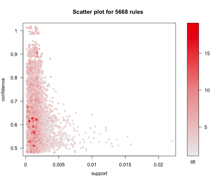
According this scatter plot, we find that support values of association analysis in general are lower, confidence values are well-distributed, and lift values of most rules are greater than 3. So these rule are significant.
Grouped matrix plot
Grouped matrix plot cluster similar rules, then shows the general distribution of clustered rules. Be default, number of cluster is 20, here I set to 15.
plot(rules, method = "grouped", control = list(k = 15))
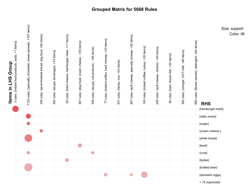
Similar association rules are grouped into one cluster, which can extract the overall regularities and similarities of association rules. Horizontal ordinate stands for 15 clusters, vertical ordinate stands for the items generated by 15 rules. The depth of color presents the degree of lift, the deeper color is, the larger lift is. The size of circle presents the degree of support, the bigger circle is, the larger support is.
Graph plot
library(igraph)
library(visNetwork)

subrules <- head(sort(rules, by = "lift"), 10)
plot(subrules, method = "graph")
Since there are enormous rules, here I just take 10 rules whose lifts are 10 largest, to make graph plot.
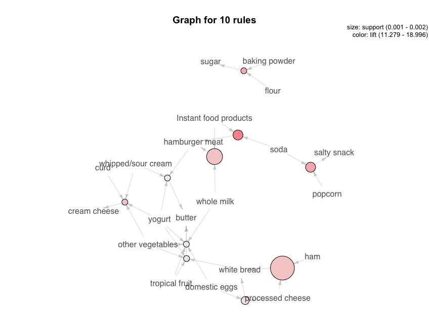
In this graph, resource means antecedent (LHS), arrow means relation direction, the circle between them means the confidence of this rule. The bigger circle is, the larger confidence is. The depth of color means the lift, the deeper color is, the larger lift is. The end of arrow pointing means the consequent (RHS) of this rule.
Following codes create a dynamic graph which is similar as above.
graphDF <- get.data.frame(plot(subrules, method = "graph"), what = "both")
visNetwork(
  nodes <- data.frame(id = graphDF$vertices$name,
                      value = graphDF$vertices$support,
                      title = ifelse(graphDF$vertices$label == "",
                                     graphDF$vertices$name,
                                     graphDF$vertices$label),
                      graphDF$vertices),
  edges <- graphDF$edges
) %>%
visOptions(highlightNearest = TRUE)How to understand this graph? Let’s take “yogurt” as an example. Click circle “yogurt”, then the circle is linked with other 4 circles, 3 small and 1 big, each of them stands for a basket. We can take the biggest one, click it, then we find that in this basket, there are also butter, whole milk, domistic eggs, tropical fruits and other vegetables. So we can say that all these products are associated with yogurt.
Association analysis is a useful way to analyse the relation between 2 different products, which can also help the decision of retailing.
Reference
- Junjie Xu, “assorted bottles and cans in commercial coolers”, www.pexels.com. [Online]. Available: https://www.pexels.com/photo/assorted-bottles-and-cans-in-commercial-coolers-3028500/